Areatangens hyperbolicus und Areakotangens hyperbolicus sind die Umkehrfunktionen von Tangens hyperbolicus und Kotangens hyperbolicus und damit Area-Funktionen .
Schreibweisen:
y
=
artanh
(
x
)
=
tanh
−
1
(
x
)
{\displaystyle y=\operatorname {artanh} (x)=\tanh ^{-1}(x)}
y
=
arcoth
(
x
)
=
coth
−
1
(
x
)
{\displaystyle y=\operatorname {arcoth} (x)=\coth ^{-1}(x)}
Letztere wird seltener benutzt, um die Verwechslung mit dem Kehrwert des hyperbolischen (Ko-)Tangens zu vermeiden. Es gilt:
artanh
(
x
)
=
tanh
−
1
(
x
)
≠
tanh
(
x
)
−
1
=
1
tanh
(
x
)
{\displaystyle \operatorname {artanh} (x)=\tanh ^{-1}(x)\not =\tanh(x)^{-1}={\frac {1}{\tanh(x)}}}
Oft werden genau bei der Umkehrfunktion auch Spitzklammern um die Minus Eins geschrieben, um diese Verwechselung zu verhindern.
Definition
Areatangens hyperbolicus und Areakotangens hyperbolicus sind folgendermaßen definiert:[ 1]
artanh
(
x
)
:=
1
2
ln
(
1
+
x
1
−
x
)
f
u
¨
r
|
x
|
<
1
{\displaystyle \operatorname {artanh} (x):={\frac {1}{2}}\ln \left({\frac {1+x}{1-x}}\right)\quad \mathrm {f{\ddot {u}}r} \quad |x|<1}
arcoth
(
x
)
:=
1
2
ln
(
x
+
1
x
−
1
)
f
u
¨
r
|
x
|
>
1
{\displaystyle \operatorname {arcoth} (x):={\frac {1}{2}}\ln \left({\frac {x+1}{x-1}}\right)\quad \mathrm {f{\ddot {u}}r} \quad |x|>1}
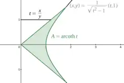
Die
arcoth
{\displaystyle \operatorname {arcoth} }
t
{\displaystyle t}
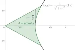
Die
artanh
{\displaystyle \operatorname {artanh} }
t
{\displaystyle t}
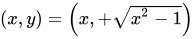
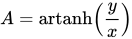
Geometrisch lässt sich der Areatangens hyperbolicus deuten als die Fläche in der Ebene, die von der Verbindungsstrecke zwischen dem Koordinatenursprung
(
0
,
0
)
{\displaystyle (0,0)}
(
x
,
y
)
{\displaystyle (x,y)}
x
2
−
y
2
=
1
{\displaystyle x^{2}-y^{2}=1}
(
x
,
−
y
)
=
(
x
,
−
x
2
−
1
)
{\displaystyle (x,-y)=\left(x,-{\sqrt {x^{2}-1}}\right)}
(
x
,
y
)
=
(
x
,
+
x
2
−
1
)
{\displaystyle (x,y)=\left(x,+{\sqrt {x^{2}-1}}\right)}
A
=
artanh
(
y
x
)
{\displaystyle A=\operatorname {artanh} \left({\frac {y}{x}}\right)}
Eigenschaften
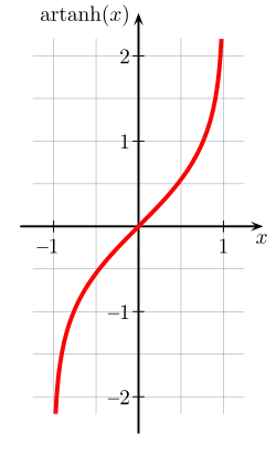
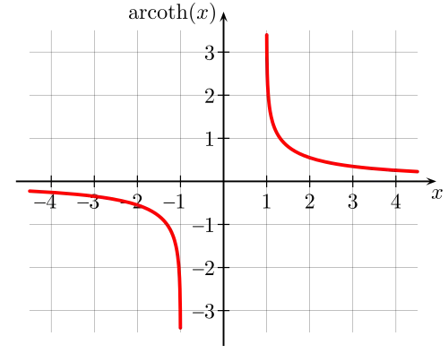
Graph der Funktion artanh(x) Graph der Funktion arcoth(x)
Areatangens hyperbolicus
Areakotangens hyperbolicus
Definitionsbereich
−
1
<
x
<
1
{\displaystyle -1<x<1}
−
∞
<
x
<
−
1
{\displaystyle -\infty <x<-1}
1
<
x
<
∞
{\displaystyle 1<x<\infty }
Wertebereich
−
∞
<
f
(
x
)
<
∞
{\displaystyle -\infty <f(x)<\infty }
−
∞
<
f
(
x
)
<
∞
;
f
(
x
)
≠
0
{\displaystyle -\infty <f(x)<\infty ;\;f(x)\neq 0}
Periodizität
keine
keine
Monotonie
streng monoton steigend
keine
Symmetrien
ungerade Funktion:
f
(
−
x
)
=
−
f
(
x
)
{\displaystyle f(-x)=-f(x)}
ungerade Funktion:
f
(
−
x
)
=
−
f
(
x
)
{\displaystyle f(-x)=-f(x)}
Asymptoten
x
=
1
:
f
(
x
)
→
∞
für
x
→
1
{\displaystyle x=1\colon \,f(x)\to \infty {\text{ für }}x\to 1}
x
=
−
1
:
f
(
x
)
→
−
∞
für
x
→
−
1
{\displaystyle x=-1\colon \,f(x)\to -\infty {\text{ für }}x\to -1}
y
=
0
:
f
(
x
)
→
0
für
x
→
±
∞
{\displaystyle y=0\colon \,f(x)\to 0{\text{ für }}x\to \pm \infty }
Nullstellen
x
=
0
{\displaystyle x=0}
keine
Sprungstellen
keine
keine
Polstellen
x
=
±
1
{\displaystyle x=\pm 1}
x
=
±
1
{\displaystyle x=\pm 1}
Extrema
keine
keine
Wendepunkte
x
=
0
{\displaystyle x=0}
keine
Reihenentwicklungen
Die Taylorreihe der Funktion
artanh
{\displaystyle \operatorname {artanh} }
[ 2]
artanh
(
x
)
=
∑
k
=
0
∞
x
2
k
+
1
2
k
+
1
=
x
+
1
3
x
3
+
1
5
x
5
+
1
7
x
7
+
⋯
{\displaystyle \operatorname {artanh} (x)=\sum _{k=0}^{\infty }{\frac {x^{2k+1}}{2k+1}}=x+{\frac {1}{3}}x^{3}+{\frac {1}{5}}x^{5}+{\frac {1}{7}}x^{7}+\dotsb }
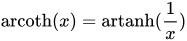
Durch Verwendung von
arcoth
(
x
)
=
artanh
(
1
x
)
{\displaystyle \operatorname {arcoth} (x)=\operatorname {artanh} ({\frac {1}{x}})}
|
x
|
>
1
{\displaystyle |x|>1}
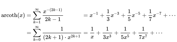
Laurent-Reihe der Funktion
arcoth
{\displaystyle \operatorname {arcoth} }
arcoth
(
x
)
=
∑
k
=
1
∞
x
−
(
2
k
−
1
)
2
k
−
1
=
x
−
1
+
1
3
x
−
3
+
1
5
x
−
5
+
1
7
x
−
7
+
⋯
=
∑
k
=
0
∞
1
(
2
k
+
1
)
⋅
x
2
k
+
1
=
1
x
+
1
3
x
3
+
1
5
x
5
+
1
7
x
7
+
⋯
{\displaystyle {\begin{alignedat}{2}\\\operatorname {arcoth} (x)&=\sum _{k=1}^{\infty }{\frac {x^{-(2k-1)}}{2k-1}}&&=x^{-1}+{\frac {1}{3}}x^{-3}+{\frac {1}{5}}x^{-5}+{\frac {1}{7}}x^{-7}+\dotsb &{}\\&=\sum _{k=0}^{\infty }{\frac {1}{(2k+1)\cdot x^{2k+1}}}&&={\frac {1}{x}}+{\frac {1}{3x^{3}}}+{\frac {1}{5x^{5}}}+{\frac {1}{7x^{7}}}+\dotsb &{}\end{alignedat}}}
Ableitungen
d
d
x
artanh
(
x
)
=
1
1
−
x
2
;
|
x
|
<
1
{\displaystyle {\frac {\mathrm {d} }{\mathrm {d} x}}\operatorname {artanh} (x)={\frac {1}{1-x^{2}}}\,;\quad |x|<1}
d
d
x
arcoth
(
x
)
=
1
1
−
x
2
;
|
x
|
>
1
{\displaystyle {\frac {\mathrm {d} }{\mathrm {d} x}}\operatorname {arcoth} (x)={\frac {1}{1-x^{2}}}\,;\quad |x|>1}
Integrale
Die Stammfunktionen von Areatangens hyperbolicus und Areakotangens hyperbolicus lauten:[ 3]
∫
artanh
(
x
)
d
x
=
x
⋅
artanh
(
x
)
+
1
2
ln
(
1
−
x
2
)
+
C
{\displaystyle \int \operatorname {artanh} (x)\,\mathrm {d} x=x\cdot \operatorname {artanh} (x)+{\frac {1}{2}}\ln \left(1-x^{2}\right)+C}
∫
arcoth
(
x
)
d
x
=
x
⋅
arcoth
(
x
)
+
1
2
ln
(
x
2
−
1
)
+
C
{\displaystyle \int \operatorname {arcoth} (x)\,\mathrm {d} x=x\cdot \operatorname {arcoth} (x)+{\frac {1}{2}}\ln \left(x^{2}-1\right)+C}
Kardinalische Areafunktionen
Weder der kardinalische Areatangens hyperbolicus noch sein Kehrwert sind mit elementaren Stammfunktionen integrierbar.
Aber die Integrale von Null bis Eins des kardinalischen Areatangens hyperbolicus sowie vom Kehrwert dieser Funktion sind beide elementar darstellbar.
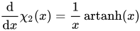
Die Ursprungsstammfunktion des Areatangens hyperbolicus cardinalis ist die Legendresche Chifunktion zum Index Zwei:
d
d
x
χ
2
(
x
)
=
1
x
artanh
(
x
)
{\displaystyle {\frac {\mathrm {d} }{\mathrm {d} x}}\chi _{2}(x)={\frac {1}{x}}\operatorname {artanh} (x)}
∫
0
x
1
y
artanh
(
y
)
d
y
=
χ
2
(
x
)
=
∫
0
1
arcsin
(
x
z
)
1
−
z
2
d
z
{\displaystyle \int _{0}^{x}{\frac {1}{y}}\operatorname {artanh} (y)\,\mathrm {d} y=\chi _{2}(x)=\int _{0}^{1}{\frac {\arcsin(xz)}{\sqrt {1-z^{2}}}}\,\mathrm {d} z}
∫
0
x
artanh
(
y
)
y
1
−
y
2
d
y
=
2
χ
2
(
x
1
+
1
−
x
2
)
{\displaystyle \int _{0}^{x}{\frac {\operatorname {artanh} (y)}{y{\sqrt {1-y^{2}}}}}\,\mathrm {d} y=2\,\chi _{2}{\biggl (}{\frac {x}{1+{\sqrt {1-x^{2}}}}}{\biggr )}}
Mit dem Kürzel
arcsin
{\displaystyle \arcsin }
Arkussinus dargestellt.
Beispielwerte
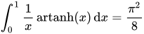
Beispielsweise gelten diese Werte:
∫
0
1
1
x
artanh
(
x
)
d
x
=
π
2
8
{\displaystyle \int _{0}^{1}{\frac {1}{x}}\operatorname {artanh} (x)\,\mathrm {d} x={\frac {\pi ^{2}}{8}}}
∫
0
1
artanh
(
x
)
x
1
−
x
2
d
x
=
π
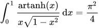
2
4
{\displaystyle \int _{0}^{1}{\frac {\operatorname {artanh} (x)}{x{\sqrt {1-x^{2}}}}}\,\mathrm {d} x={\frac {\pi ^{2}}{4}}}
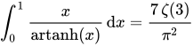
Wenn der Kehrwert des Areatangens hyperbolicus cardinalis von Null bis Eins integriert wird, dann entsteht das Siebenfache der Apéry-Konstante dividiert durch das Quadrat der Kreiszahl :
∫
0
1
x
artanh
(
x
)
d
x
=
7
ζ
(
3
)
π
2
{\displaystyle \int _{0}^{1}{\frac {x}{\operatorname {artanh} (x)}}\,\mathrm {d} x={\frac {7\,\zeta (3)}{\pi ^{2}}}}
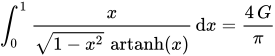
Wenn der Kehrwert des Areatangens hyperbolicus cardinalis durch die pythagoräische Gegenstückfunktion geteilt wird, dann entsteht das Vierfache der Catalan-Konstante dividiert durch die Kreiszahl:
∫
0
1
x
1
−
x
2
artanh
(
x
)
d
x
=
4
G
π
{\displaystyle \int _{0}^{1}{\frac {x}{{\sqrt {1-x^{2}}}\,\operatorname {artanh} (x)}}\,\mathrm {d} x={\frac {4\,G}{\pi }}}
Wenn der Kehrwert vom Quadrat des Areatangens hyperbolicus cardinalis von Null bis Eins integriert wird, dann entsteht folgender Wert:
∫
0
1
x
2
artanh
(
x
)
2
d
x
=
1
3
π
4
[
372
ζ
(
5
)
−
14
π
2
ζ
(
3
)
]
{\displaystyle \int _{0}^{1}{\frac {x^{2}}{\operatorname {artanh} (x)^{2}}}\,\mathrm {d} x={\frac {1}{3\,\pi ^{4}}}{\bigl [}372\,\zeta (5)-14\,\pi ^{2}\zeta (3){\bigr ]}}
Additionstheoreme
artanh
(
x
)
±
artanh
(
y
)
=
artanh
(
x
±
y
1
±
x
y
)
{\displaystyle \operatorname {artanh} (x)\pm \operatorname {artanh} (y)=\operatorname {artanh} \left({\frac {x\pm y}{1\pm xy}}\ \right)}
[ 1]
arcoth
(
x
)
±
arcoth
(
y
)
=
arcoth
(
1
±
x
y
x
±
y
)
{\displaystyle \operatorname {arcoth} (x)\pm \operatorname {arcoth} (y)=\operatorname {arcoth} \left({\frac {1\pm xy}{x\pm y}}\ \right)}
Umrechnung und Beziehungen zu Arkusfunktionen
artanh
(
x
)
=
arcoth
(
1
x
)
|
x
|
<
1
{\displaystyle \operatorname {artanh} (x)=\operatorname {arcoth} \left({\frac {1}{x}}\right)\quad |x|<1}
arcoth
(
x
)
=
artanh
(
1
x
)
|
x
|
>
1
{\displaystyle \operatorname {arcoth} (x)=\operatorname {artanh} \left({\frac {1}{x}}\right)\quad |x|>1}
artanh
(
z
)
=
−
i
arctan
(
i
z
)
{\displaystyle \operatorname {artanh} (z)=-i\arctan(iz)}
arcoth
(
z
)
=
i
arccot
(
i
z
)
{\displaystyle \operatorname {arcoth} (z)=i\operatorname {arccot}(iz)}
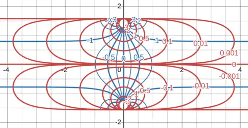
Komplexe Transformation
x
+
i
y
=
artanh
(
u
+
i
v
)
{\displaystyle x+iy=\operatorname {artanh} (u+iv)}
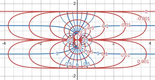
Komplexe Transformation
x
+
i
y
=
arcoth
(
u
+
i
v
)
{\displaystyle x+iy=\operatorname {arcoth} (u+iv)}
Siehe auch
Weblinks
Einzelnachweise
↑ a b Ilʹja N. Bronštejn: Taschenbuch der Mathematik . 11., aktualisierte Auflage. Haan-Gruiten 2020, ISBN 978-3-8085-5792-1, S. 95 .
↑ Ilʹja N. Bronštejn: Taschenbuch der Mathematik . 11., aktualisierte Auflage. Haan-Gruiten 2020, ISBN 978-3-8085-5792-1, S. 1080 .
↑ Ilʹja N. Bronštejn: Taschenbuch der Mathematik . 11., aktualisierte Auflage. Haan-Gruiten 2020, ISBN 978-3-8085-5792-1, S. 1116 (Formeln 514, 515).






























![{\displaystyle \int _{0}^{1}{\frac {x^{2}}{\operatorname {artanh} (x)^{2}}}\,\mathrm {d} x={\frac {1}{3\,\pi ^{4}}}{\bigl [}372\,\zeta (5)-14\,\pi ^{2}\zeta (3){\bigr ]}}](./_assets_/eb734a37dd21ce173a46342d1cc64c92/0b5b145a44114ae4c0145b10e92c2fcdee54ed4c.svg)